Getting Started

Welcome to Modular Diffusion! This tutorial highlights the core features of the package and will put you on your way to prototype and train your own Diffusion Models. For more advanced use cases and further details, check out our other tutorials and the library’s API reference.

Prerequisites

This tutorial assumes basic familiarity with Diffusion Models. If you are just hearing about Diffusion Models, you can find out more in one of the many tutorials out there.

Install the package

Before you start, please install Modular Diffusion in your local Python environment by running the following command:

python -m pip install modular-diffusion

Additionally, ensure you’ve installed the correct Pytorch distribution for your system.

Train a simple model

The first step before training a Diffusion Model is to load your dataset. In this example, we will be using MNIST, which includes 70,000 grayscale images of handwritten digits, and is a great simple dataset to prototype your image models. We are going to load MNIST with Pytorch Vision, but you can load your dataset any way you like, as long as it results in a torch.Tensor object. We are also going to discard the labels and scale the data to the commonly used $[-1, 1]$ range.

import torch
from torchvision.datasets import MNIST
from torchvision.transforms import ToTensor

x, _ = zip(*MNIST(str(input), transform=ToTensor(), download=True))
x = torch.stack(x) * 2 - 1

Let’s build our Diffusion Model next. Modular Diffusion provides you with the diffusion.Model class, which takes as parameters a data transform, a noise schedule, a noise type, a denoiser neural network, and a loss function, along with other optional parameters. You can import prebuilt components for these parameters from the different modules inside Modular Diffusion or build your own. Let’s take a look at a simple example which replicates the architecture introduced in Ho et al. (2020), using only prebuilt components:

import diffusion
from diffusion.data import Identity
from diffusion.loss import Simple
from diffusion.net import UNet
from diffusion.noise import Gaussian
from diffusion.schedule import Linear

model = diffusion.Model(
    data=Identity(x, batch=128, shuffle=True),
    schedule=Linear(1000, 0.9999, 0.98),
    noise=Gaussian(parameter="epsilon", variance="fixed"),
    net=UNet(channels=(1, 64, 128, 256)),
    loss=Simple(parameter="epsilon"),
    device="cuda" if torch.cuda.is_available() else "cpu",
)

You might have noticed that we also added a device parameter to the model, which is important if you’re looking to train on the GPU. We are now all set to train and sample from the model. We will train the model for 20 epochs and sample 10 images from it.

losses = [*model.train(epochs=20)]
z = model.sample(batch=10)

Tip

If you are getting a Process killed message when training your model, try reducing the batch size in the data module. This error is caused by running out of RAM.

The sample function returns a tensor with the same shape as the dataset tensor, but with an extra diffusion time dimension. In this case, the dataset has shape [b, c, h, w], so our output z has shape [t, b, c, h, w]. Now we just need to rearrange the dimensions of the output tensor to produce one final image.

from einops import rearrange
from torchvision.utils import save_image

z = z[torch.linspace(0, z.shape[0] - 1, 10).int()]
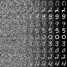
z = rearrange(z, "t b c h w -> c (b h) (t w)")
save_image((z + 1) / 2, "output.png")

And that’s it! The image we just saved should look something like this:

Random numbers being generated from noise.

Add a validation loop

You might have noticed that the train method returns a generator object. This is to allow you to validate the model between epochs inside a for loop. For instance, you can see how your model is coming along by sampling from it between each training epoch, rather than only at the end.

for epoch, loss in enumerate(model.train(epochs=20)):
    z = model.sample(batch=10)
    z = z[torch.linspace(0, z.shape[0] - 1, 10).int()]
    z = rearrange(z, "t b c h w -> c (b h) (t w)")
    save_image((z + 1) / 2, f"{epoch}.png")

Tip

If you’re only interested in seeing the final results, sample the model with the following syntax: *_, z = model.sample(batch=10). In this example, this will yield a tensor with shape [b, c, h, w] containing only the generated images.

Swap modules

The beauty in Modular Diffusion is how easy it is to make changes to an existing model. To showcase this, let’s plug in the Cosine schedule introduced in Nichol & Dhariwal (2021). All it does is destroy information at a slower rate in the forward diffusion process, which was shown to improve sample quality.

from diffusion.schedule import Cosine

model = diffusion.Model(
    data=Identity(x, batch=128, shuffle=True),
    schedule=Cosine(steps=1000), # changed the schedule!
    noise=Gaussian(parameter="epsilon", variance="fixed"),
    net=UNet(channels=(1, 64, 128, 256)),
    loss=Simple(parameter="epsilon"),
    device="cuda" if torch.cuda.is_available() else "cpu",
)

By keeping the rest of the code the same, we end up with the following result:

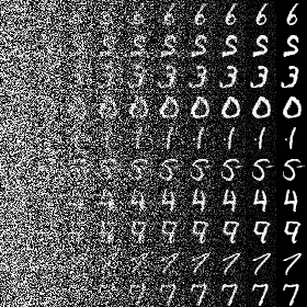
Random numbers being generated from noise at a slower rate.

You can see that, because we used the cosine schedule, the denoising process is more gradual compared to the previous example.

Train a conditional model

In most Diffusion Model applications, you’ll want to be able to condition the generation process. To show you how you can do this in Modular Diffusion, we’ll continue working with the MNIST dataset, but this time we want to be able to control what digits we generate. Like before, we’re going to load and preprocess the dataset, but this time we want to keep the labels, which tell us what number is in each image. We are also going to move the labels one unit up, since the label 0 is reserved for the null class.

x, y = zip(*MNIST(str(input), transform=ToTensor(), download=True))
x, y = torch.stack(x) * 2 - 1, torch.tensor(y) + 1

Once again, let’s assemble our Diffusion Model. This time, we will add the labels y in our data transform object and provide the number of labels to our denoiser network. Let’s also add classifier-free guidance to the model, a technique introduced in Ho et al. (2022) to improve sample quality in conditional generation, at the cost of extra sample time and less sample variety.

from diffusion.guidance import ClassifierFree

model = diffusion.Model(
    data=Identity(x, y, batch=128, shuffle=True), # added y in here!
    schedule=Cosine(steps=1000),
    noise=Gaussian(parameter="epsilon", variance="fixed"),
    net=UNet(channels=(1, 64, 128, 256), labels=10), # added labels here!
    guidance=ClassifierFree(dropout=0.1, strength=2), # added classifier guidance!
    loss=Simple(parameter="epsilon"),
    device="cuda" if torch.cuda.is_available() else "cpu",
)

One final change we will be making compared to our previous example is to provide the labels of the images we wish to generate to the sample function. As an example, let’s request one image of each digit by replacing model.sample(batch=10) with model.sample(y=torch.arange(1, 11)). We then end up with the following image:

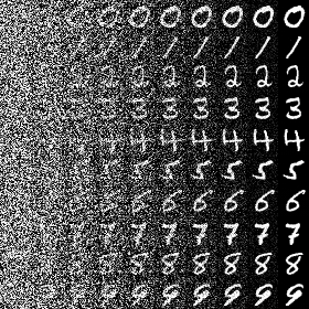
Numbers 0 through 9 being generated from noise.

Pretty cool, uh? You can see how now we can choose which digit we sample from the model. This is, of course, only the tip of the iceberg. If you are looking more advanced conditioning techniques, such as the one used in DALL·E 2, please refer to our Image Generation Guide.

Save and load the model

Once you’re done training your Diffusion Model, you may wish to store it for later. Modular Diffusion provides you with an intuitive interface to achieve this. Below is the syntax for saving the model:

model.save("model.pt")

In order to load it back, use the following snippet:

from pathlib import Path

if Path("model.pt").exists()
	model.load("model.pt")

Remember to always initialize the model prior to loading it, preferably with the same parameters you trained the model with. The load function will then populate the model weights with the ones you have saved.

Warning

In some scenarios, you might want to introduce changes to the model architecture before you load it in. In these cases, it is important to keep in mind that structures that hold trainable weights, like the net parameter, cannot be changed, or your script will crash. Moreover, your Diffusion Model will most likely need to be trained for a few additional epochs if you make any changes to its parameters.

Create your own modules

As you’ve seen, Modular Diffusion provides you with a library of prebuilt modules you can plug into and out of your model according to your needs. Sometimes, however, you may need to customize the model behavior beyond what the library already offers. To address this, each module type has an abstract base class, which serves as a blueprint for new modules. To create your own custom module, simply inherit from the base class and implement the required methods.

Suppose, for example, you want to implement your own custom noise schedule. You can achieve this by extending the abstract Schedule base class and implement its only abstract method, compute. This method is responsible for providing a tensor containing the values for $\alpha_t$ for $t \in \{0,\dots,T\}$ . As an example, let’s reimplement the Linear schedule:

from dataclasses import dataclass
from diffusion.base import Schedule

@dataclass
class Linear(Schedule):
    start: float
    end: float

    def compute(self) -> Tensor:
        return torch.linspace(self.start, self.end, self.steps + 1)

Given that steps is already a parameter in the base class, all we need to do is define start and end parameters, and use them to compute the $a_t$ values. Now you can use your custom module in your diffusion.Model just like you did with the prebuilt ones! For more detailed guidance on extending each module type check out our Custom Modules Tutorial.

Another neat feature of Modular Diffusion is it provides an intuitive way to combine existing modules without having to create new ones. For instance, sometimes you’ll want to train the model on a hybrid loss function that is a linear combination of two or more functions. In their paper, Nichol & Dhariwal (2021) introduced such a loss function, which is a linear combination of the simple loss function proposed by Ho et al. (2020) and the variational lower bound (VLB):

$L_\text{hybrid}=L_\text{simple}+0.001 \cdot L_\text{vlb}$

With Modular Diffusion, rather than creating a custom hybrid loss module, you can conveniently achieve this by combining the Simple and VLB modules:

from diffusion.loss import Simple, VLB

loss = Simple(parameter="epsilon") + 0.001 * VLB()

Similarly, you can append post-processing layers to your denoiser network with the pipe operator, without the need to create a new Net module:

from diffusion.net import Transformer
from torch.nn import Softmax

net = Transformer(input=512) | Softmax(2)

If you spot any typo or technical imprecision, please submit an issue or pull request to the library's GitHub repository .